MachineKit LTTng kernel trace

How does MachineKit execution look like at the system level? Here are some observations done using an LTTng kernel trace on Linux preempt-rt 4.1.13-rt15 on a 4 cores machine. The workload traced is the abs.0 unit test. This test spawns halcmd, simulating the position control of a motor (or something). Here is the command:

cd machinekit/
. scripts/rip-environment
cd tests/abs.0/
halcmd -v test.hal

The overall command takes 3.3s to complete. Let's check what's in the trace.

First, the rtapi processing takes about 600ms to execute and is shown in Figure 1. One of the related process, named fast:0, seems to do the actual real-time job and is shown in Figure 2. This process sleeps periodically using the system call clock_nanosleep(). I observed a wake-up latency of about 30us and the thread itself runs for about 2-3us in user-space before returning to sleep.

Figure 1: Overview of the rtapi execution.

Figure 2: Real-time process with period of about 300us.

The scripts and utilities to manage the test environment behave quite differently than the RT process. In particular, there is a bunch of processes that interact for very short durations, namely halcmd and rtapi, as shown in Figure 3. They perform sendto() and recvfrom() system calls, probably for round-trip communication. Maybe using shared memory could help here to streamline the communication. There is numerous sleep of 10ms to 200ms performed by halcmd in midway. 

Figure 3: Interactions between halcmd and rtapi.

There is a pattern of fork-exec-wait done by the script realtime shown in Figure 4. This script spawns inivar, flavor and halrun executables, together running for more than 400ms. Using programmatic API instead of spawning executables would make the processing more efficient. 

Figure 4: Repeated fork-exec-wait pattern.

Finally, there is a giant 2.5s sleep at the end of the test, shown in Figure 5. It represents therefore 75% of the test execution time. This kind of sleep is usually done for quick-n-dirty synchronization, but should be replaced by wait for the actual event required to execute as quickly as possible. This way, the time to run the unit tests can be decreased significantly, possibly representing greater productivity for developers.

Of course, if we had a user-space trace in addition to the kernel trace, we could have a greater insight of the internal state of machinekit. But even without, we can observe interesting behavior. The next step will be to actually plug and control some actual hardware in real-time.

Why malware detection based on syscalls n-grams is unlikely to work

In the field of computer security, it was suggested to use n-grams of system calls to detect malware running on a computer. Let's demonstrate that there is no relationship between n-gram counts and malicious behavior.

False-negative example. The first trace is a weather app that opens a config file, then performs some remote procedure call to get the data, and then closes file descriptors. The other is the same sequence, but for a malicious app that gained root privilege by some means, and sends the content of the password file.

Trace A1: open(“app.conf”); read(); connect(); send(); recv(); close(); close()

Trace A2: open(“/etc/passwd”); read(); connect(); send(); recv(); close(); close()

The probability of each n-gram is trivially the same for the same sequence. Therefore, the algorithm fails to detect the malware.

False-positive example. Both sequences are functionally equivalent and non-malicious, but the second trace reduces the maximum number of opened file descriptor at one time.

Trace B1: open(); open(); open(); read(); read(); read(); close(); close(); close()

Trace B2: open(); read(); close(); open(); read(); close(); open(); read(); close()

Let’s use Python to generate all n-grams of size 3.

ngrams = [x for x in itertools.product(['open','read','close'],['open','read','close'],['open','read','close'])]

                                        B1 B2 (B2 sym diff B1)

open  open  open  1 0  \empty
open  open  read  1 0  \empty
open  open close  0 0
open  read  open  0 0
open  read  read  1 0  \empty
open  read close  0 3  \empty
open close  open  0 0
open close  read  0 0
open close close  0 0
read  open  open  0 0
read  open  read  0 0
read  open close  0 0
read  read  open  0 0
read  read  read  1 0  \empty
read  read close  1 0  \empty
read close  open  0 2  \empty
read close  read  0 0
read close close  1 0  \empty
close  open  open  0 0
close  open  read  0 2  \empty
close  open close  0 0
close  read  open  0 0
close  read  read  0 0
close  read close  0 0
close close  open  0 0
close close  read  0 0
close close close  1 0  \empty

total              7 7

The n-gram counts for both sets are totally disjoints. Therefore, the algorithm will wrongly detect the trace B2 as malware code, while it is in fact the result of a simple optimization.

Moreover, a malicious app can trick the detection by calling dummy system calls randomly, which will swamp the potentially mallicious sequences. Because each n-gram probability will be non-statistically significant, the algorithm will fail to identify the change of behavior, and classify it as malware.

Therefore, we conclude that this technique is unlikely to provide any benefits to identify malware automatically.

Full stack Python tracing

The project profile-python-ust allows to record function call and return from Python interpreted code using LTTng-UST. As an example, consider this foo.py code (calling itself bidon.py that just print something on the console):

import bidon

def baz():
    bidon.bidon()

def bar():
    baz()

def foo():
    bar()

if __name__=='__main__':
    foo()

The trace produced is:

python:call: { cpu_id = 7 }, { co_name = "" }
python:call: { cpu_id = 7 }, { co_name = "foo" }
python:call: { cpu_id = 7 }, { co_name = "bar" }
python:call: { cpu_id = 7 }, { co_name = "baz" }
python:return: { cpu_id = 7 }, { }
python:return: { cpu_id = 7 }, { }
python:return: { cpu_id = 7 }, { }
python:return: { cpu_id = 7 }, { }

However, the tracing hooks into CPython are not called for external C modules. Therefore, we loose track of what is going on. For instance, Cython compiles Python code as a native shared library for greater efficiency. To overcome this limitation, I compiled the Cython foo.pyx code using GCC function instrumentation. Here is the setup.py file (The same code gets compiled twice, with and without instrumentation):

from distutils.core import setup
from Cython.Build import cythonize
from distutils.extension import Extension

ext = [
    Extension('foo1', ['foo1.pyx'],
              extra_compile_args = ['-g'],
    ),
    Extension('foo2', ['foo2.pyx'],
              extra_compile_args = ['-finstrument-functions', '-g'],
    ),
]

setup(
    ext_modules = cythonize(ext),
)

And then I invoked both modules foo1.foo() and foo2.foo(), with the lttng-ust-cyg-profile instrumentation, that hooks on the GCC instrumentation. I also enabled kernel tracing, just for fun. Both traces (kernel and user space) are loaded in an Trace Compass experiment.

We see in the screenshot below the users space stack according to time for the foo1 and foo2 executions. In the first execution, we see the entry point of inside foo1.so and the invocation of Python code from the library, but function calls inside foo1.so are not visible. In the second execution, both the Python and the GCC instrumentation are available, and the complete callstack is visible. The higlighted time range is about 6us and corresponds to the write() system call related to the print() on the console. We can see the system call duration and the blocking in the control flow view.

Unfortunately, symbols can't be resolved, because base address library loading can't be enabled at this time with Python instrumentation, due to this bug.

This was an example how three sources of events finally create a complete picture of the execution!

EDIT:

A Cython module can call profile hook of the main interpreter. Call cython with the profile option, and compile the resulting code with -DCYTHON_TRACE=1. This can be done in setuptools with:

 cythonize(ext_trace, compiler_directives={'profile': True}),

Thanks to Stefan Behnel for this tip!

How Linux changes the CPU Frequency

The ondemand governor adjust the processor frequency making a trade-off between power and performance, and is the implementation of Dynamic Frequency Scaling under Linux. However, it was also causing unexpected delays in my performance benchmarks. The following figure shows the delay density of RPC requests for the CPU frequency governor ondemand and performance. Delay variation is lower when the CPU frequency is fixed.

I wanted to visualize how the frequency changes according to time and scheduling. I used LTTng to record power_cpu_frequency and sched_switch events. I loaded them in Trace Compass, and defined the analysis declaratively using XML (available here). The CPU frequency is shown in shades of red (stronger means higher frequency) and in green whether the CPU is busy or idle. (you guessed correctly, holiday season is coming). We see in the following figure that it takes some time for the frequency to ramp-up.

In fact, changing the CPU frequency is equivalent to distorts the elapsed time of the execution. Timestamps in the trace are in nanoseconds instead of clock cycles, but to compare executions, the base should be clock cycles instead. We could scale the time using the frequency events to approximate the time in processor cycles.

The task kworker, woken-up from a timer softirq, changes the CPU frequency. The kworker thread runs with a varying period, typically between 4ms and 20ms. The algorithm seems to take into account the average CPU usage, because if the CPU does rapid context switch between idle and busy, the frequency never reaches the maximum.

Therefore, a task performing frequent blocking/running cycles may run faster if it shares the CPU with another task, because the average CPU usage will increase and frequency will be set accordingly. We could also estimate the relative power cost of a segment of computation with great precision.

In conclusion, disabling frequency scaling for benchmarks should reduce variability. Here is how to do it on recent Linux kernels:

set_scaling_gov() {
        gov=${1-performance}
        for i in $(ls -1 /sys/devices/system/cpu/cpu*/cpufreq/scaling_governor); do
                echo ${gov} | sudo tee $i > /dev/null
        done
}

Here is the view for the whole trace. Happy hacking!

LinuxCon 2014, Düsseldorf

Distributed Active Path from Kernel Trace

I presented recent work about the recovery of active path of a distributed program, only using a kernel trace. The result is a time-view of the execution across computers. One of the most interesting result is the Django Poll three-tiers app, including an Apache web server and a PostgreSQL database. Client is simulated by scripting with Mechanize. The screen shot shows the execution for the POST, where a large sync is visible near the end of the sequence, necessary for the update SQL statement. 

Declarative views from user-space trace with Trace Compas

Geneviève Bastien presented how to use LTTng-UST and Trace Compas to create a time view of the state of an MPI computation. The MPI program simulates unbalanced computation, where the green represent work, and red is wait at the barrier. Multiple cycles are shown, and all the views are synchronized, which is handy to analyse the application at multiple level at once. In the following figure, we see below that the wait at the barrier (in red) is actually implemented using a busy loop calling non-blocking poll() system call, shown on top. We observed this behavior with the OpenMPI library, and we think it is intended to reduce the latency at the expense of power and resource efficiency.

Below: MPI imbalance application state (green: compute, red: wait). Above: corresponding kernel trace, including a zoom on the busy wait.

Preemption analysis across host and virtual machines

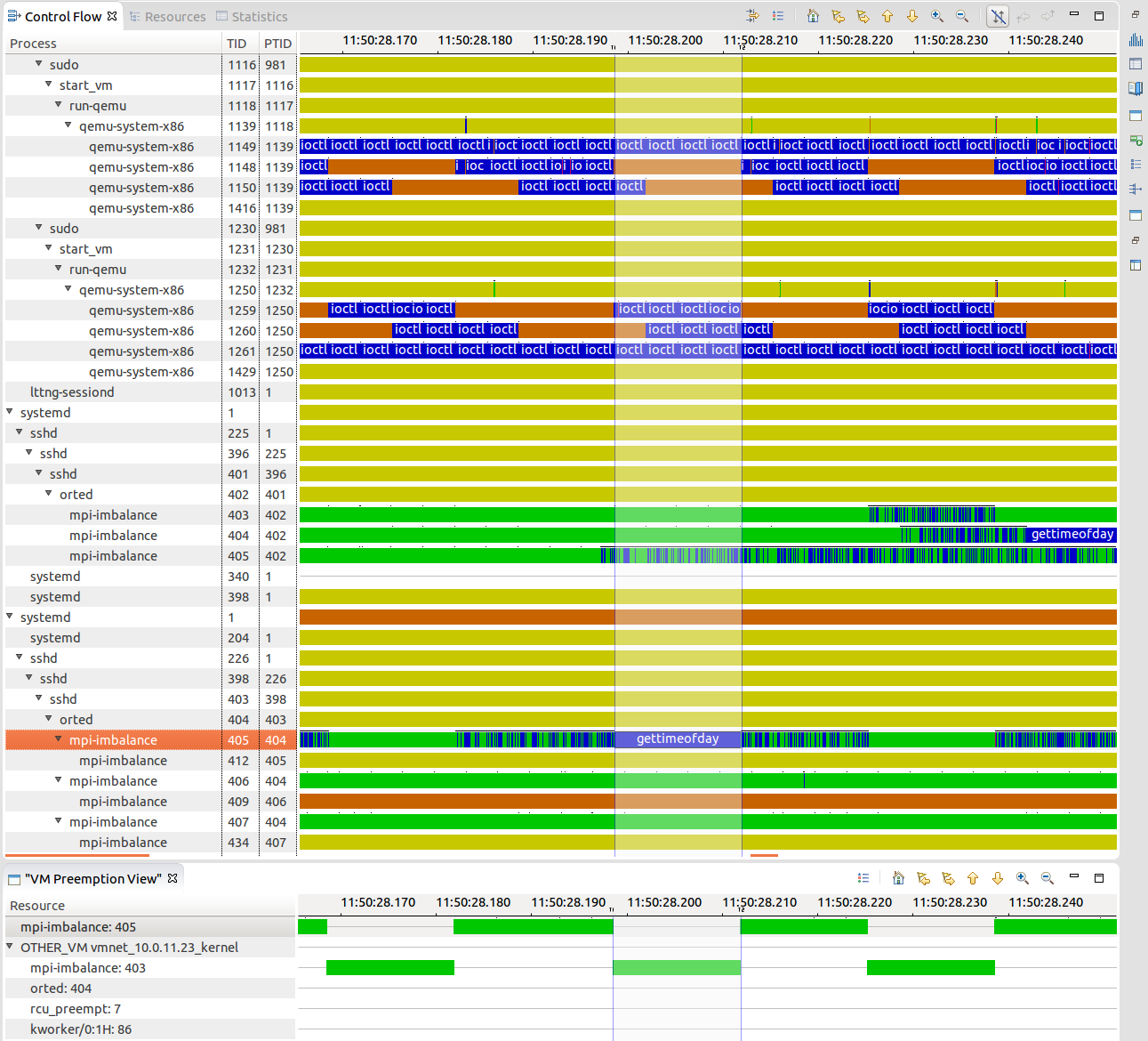
Execution in virtual machines is subject to higher level of variation in response time. Geneviève Bastien presented the virtual machine analysis, that shows the preemption crossing virtual machines boundaries, the research result of former student Mohamad Gebai. A process in the VM may appear to run while it is not, because the process representing its virtual CPU on the host is be preempted. The host and the VMs are traced at the same time, and traces are synchronized. The global view of the resources allows to pinpoint preemption cause given a task, whenever the other task is local, on the host or inside another virtual machine. The following figure shows qemu processes on the host and traces from within the host. We clearly see a gettimeofday() that is much longer that one would expect (13ms instead of ~200ns), and the reason is that there is another process, in another VM, that was running for that time, and the preemption cause is shown below.

Total view of the system, crossing virtual machine boundaries.

ftrace

Sten Rosted from RedHat presented the inner working of ftrace. It is a framework to hook into each function in the kernel. The kernel is compiled with gcc -pg option, that adds a call to mcount() at the beginning of each function, but this call is replaced by nops. The space left in each function header is patched at runtime to jump to the instrumentation. This framework is used by kprobe, but the ftrace backend can be used directly instead.

folly

Ben Maurer from Facebook presented efficiency and scalability issues they face in their environment. Performance in accepting connections is critical. He mentioned that getting the next available file descriptor is a linear search that hurts the performance. He also shows a method to decrease the number of scheduling switch of workers by replacing pthread condition wait, and improving load distribution among threads. I liked his quantitative approach, always evaluating both kernel and user-space solutions to the same problem.

Cycle accurate profiling using CoreSight hardware trace

Pawel Moll from ARM presented the CoreSight instruction tracing capabilities. The processor records branch taken and the number of cycles taken by each instructions. He demonstrated a prototype of cycle accurate (i.e. exact cycle count) profiler. The trace decoding is somewhat cumbersome, because the code memory must be reconstructed offline to resolve address symbols, and the complete toolchain requires proper integration, but still an impressive demonstration.

Thanks to NVIDIA!

I also got a JETSON TK1 big.LITTLE board from NVIDIA. I will be able to test heterogenous traces experiments (x86, arm), a very common case for mobile and cloud computing. I will also be able to test the CoreSight tracing. Thanks NVIDIA!

Ubuntu login analysis

I'm tracing a lot these days, and in the viewer, I need to scroll a lot to get to the interesting stuff in the control flow view. Today, I checked all these processes for fun. In fact, it's related to landscape triggered on Ubuntu login. To display the message about system usage and updates (which I think is great), landcape calls numerous sub-programs, for a total of about 250ms on my system. It's something one should keep in mind if SSH commands are repeated in a tight loop: the maximum rate is about 4 commands per seconds. Hopefully, Fabric reuses SSH connection! ;-)

Ubuntu login greeting

The active path of the computation of the login greeting

Pinpoint memory usage of Java program with Eclipse Memory Analyzer

My Java program was using a lot of memory. An object was holding a reference on a large temporary data structure, even after it was out of scope. It is indeed difficult to understand what prevent the garbage collection to do its job. Here is how I found out.

• Download and extract Eclipse Memory Analyzer (MAT).
• Download the HeapDump.java class and insert a call to HeapDump.dumpHeap() after the point your think the memory should be released.
• Run the instrumented program. The resulting file size may be rather large (seems to be the hole VM memory), so make sure you have enough free space.
• Open it in MAT. (Notice: I was experiencing a hang bug on Ubuntu 14.04, dismiss the initial report dialog and do not generate HTML reports, it seems to trigger the bug). Click on Dominator Tree.
• Once you found the offending object, right click on it and select Path to GC Roots > with all references. This will display the references that prevent the GC to free this object.
• Fix the code and you can start over to verify that the problem is indeed fixed ;-)

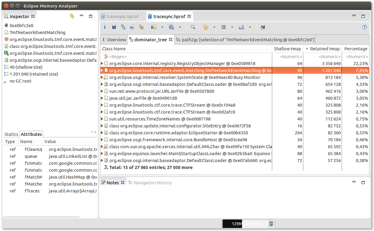
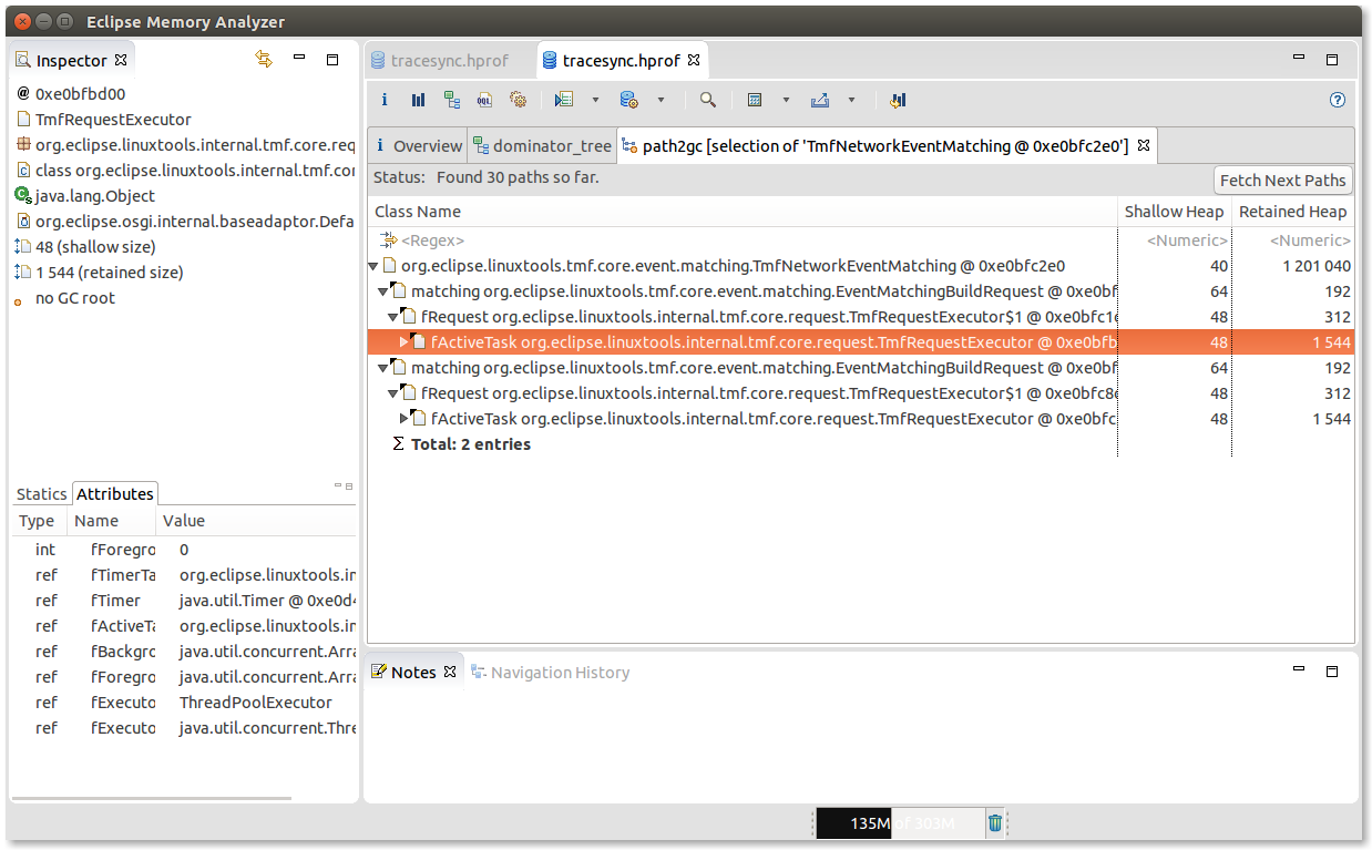
The following screenshots shows an example of the tool usage for my problem. The class TmfNetworkEventsMatching matches send to receive network events in a trace. Unmatched packets are kept temporarily in memory. However, the old unmatched packets were never freed. In the Dominator Tree, we see that TmfNetworkEventsMatching is 40 bytes (Shallow Heap), but holds around 1.2MB of objects (Retained Heap). The Path to GC Roots highlights that a reference of TmfNetworkEventMatching is kept inside TmfRequestExecutor. In this case, a missing call to dispose() was preventing the release of resources. Other resources are auto-closable, except for one of them, which needs manual call to dispose(). Thank you MAT!

Dominator Tree

Path to GC Roots